on
Blog Post 7: Unexpected Shocks
I chose gas prices as a shock of this year that I could try to quantify in order to test the relationship with support for Democrats or Republicans. The data I looked at took the nationwide average price of gas in dollars per gallon for each week of the year.
gas <- read_csv("/Users/claireduncan/Downloads/07 - Shocks (10:20)/Gas_prices_weekly.csv")

gas_week <- gas %>%
  mutate(date = mdy(date)) %>%
  mutate(year = substr(date, 1, 4)) %>%
  filter(year == 2022) %>%
  mutate(week = strftime(date, format = "%V")) %>%
  mutate(month = strftime(date, format = "%m")) %>%
  mutate(avg_change = 100*
           ((avg_gasprice - lag(avg_gasprice)) / (lag(avg_gasprice))))

gas_week$avg_change[is.na(gas_week$avg_change)] <- 0
When considering how to quantify gas prices as a shock, I looked at both the average price of gas per week in the US and then the percent change in gas price from week to week, comparing one week to the previous week. This graph shows that percent change, demonstrating the significant increase around week 20. That was when the gas prices hit a record high in June - averaging about $5 nationwide; before the average fell for 98 straight days, dropping to around $3.5 per gallon, which is demonstrated by the negative percent changes during that time frame. The decrease after the large peak increase starts around week 24 which was mid June of this year.
gas_week %>%
  ggplot(aes(x=week, y=avg_change)) +
  geom_point(color="blue") +
  theme_classic() + geom_hline(yintercept=0, color = "black", size=0.5) +
  labs(x= "Week of Year", y="Percentage Change in Gas Prices \n(from previous week)", title = "2022 Percent Change in Gas Prices (Week to Week)") + scale_y_continuous(limits=c(-5,5))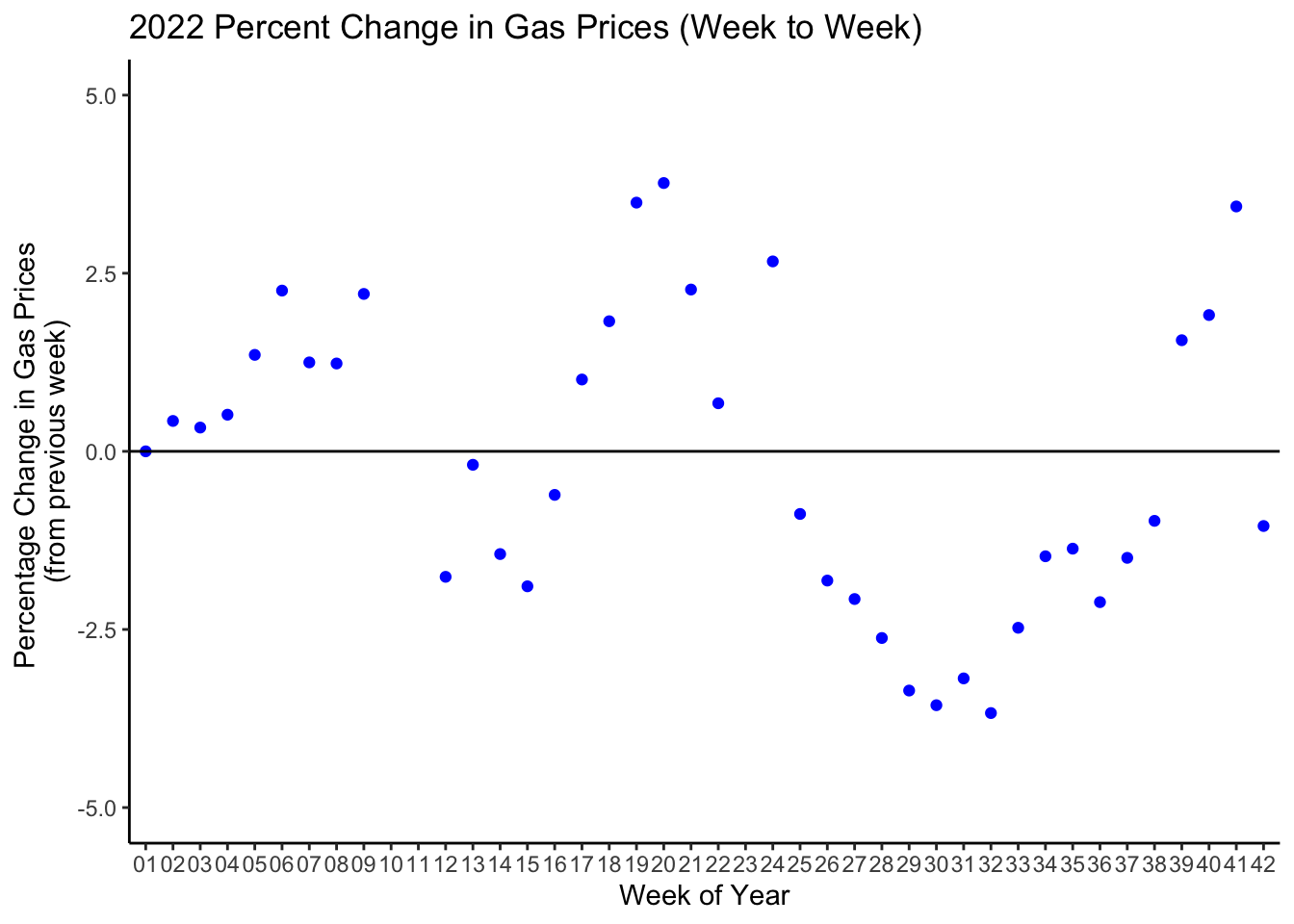
Then I created a graph using the NYT scrape of the term “gas prices” in which the most articles per week were written in early March, with other peaks in mid to late June. Noted on here are the greatest and lowest data points from the previous slide indicating increases and decreases in price change by week. It’s clear that when gas prices first increased significantly, there were the most articles written about that change.
Using the generic ballot data we have, I ran correlations between gas price and support for Democrats and Republicans. Only looking at the weekly price of gas, an increase in dollar per gallon was associated with a very small increase in support for both Democrats and Republicans although this was only statistically significant for Republican generic ballot support.
Then, I looked at the average change in price, comparing each week to the previous week. I thought this might be a better indicator of how gas prices have been a “shock” considering how people make quick retrospective comparisons in how much they have to pay week to week. This measure was greater and more significant for both democratic and republican support. For Democrats, an increase in gas price change was correlated with a decrease in support of almost 1%. Meanwhile for Republicans, an increase in gas price change was correlated with an increase in support of 0.8%. This seems to be indicative of not only how Republicans have used gas prices to attack Democrats and fire up their base, but of how voters use the logic of retrospection - holding the incumbent Democrats responsible for the sharp increases in gas prices this summer.
gas_Dem <- lm(avg_support ~ avg_gasprice, data = gas_comp_Dem)
stargazer(gas_Dem, type='text')
##
## ===============================================
## Dependent variable:
## ---------------------------
## avg_support
## -----------------------------------------------
## avg_gasprice 0.073
## (0.099)
##
## Constant 42.647***
## (0.406)
##
## -----------------------------------------------
## Observations 262
## R2 0.002
## Adjusted R2 -0.002
## Residual Std. Error 0.806 (df = 260)
## F Statistic 0.553 (df = 1; 260)
## ===============================================
## Note: *p<0.1; **p<0.05; ***p<0.01gas_Dem2 <- lm(avg_support ~ avg_change, data = gas_comp_Dem)
stargazer(gas_Dem2, type='text')##
## ===============================================
## Dependent variable:
## ---------------------------
## avg_support
## -----------------------------------------------
## avg_change -0.095***
## (0.014)
##
## Constant 42.980***
## (0.046)
##
## -----------------------------------------------
## Observations 262
## R2 0.145
## Adjusted R2 0.141
## Residual Std. Error 0.746 (df = 260)
## F Statistic 43.975*** (df = 1; 260)
## ===============================================
## Note: *p<0.1; **p<0.05; ***p<0.01gas_Rep <- lm(avg_support ~ avg_gasprice, data = gas_comp_Rep)
stargazer(gas_Rep, type='text')##
## ===============================================
## Dependent variable:
## ---------------------------
## avg_support
## -----------------------------------------------
## avg_gasprice 0.872***
## (0.075)
##
## Constant 40.840***
## (0.309)
##
## -----------------------------------------------
## Observations 262
## R2 0.342
## Adjusted R2 0.339
## Residual Std. Error 0.613 (df = 260)
## F Statistic 135.075*** (df = 1; 260)
## ===============================================
## Note: *p<0.1; **p<0.05; ***p<0.01gas_Rep2 <- lm(avg_support ~ avg_change, data = gas_comp_Rep)
stargazer(gas_Rep2, type='text')##
## ===============================================
## Dependent variable:
## ---------------------------
## avg_support
## -----------------------------------------------
## avg_change 0.081***
## (0.014)
##
## Constant 44.375***
## (0.044)
##
## -----------------------------------------------
## Observations 262
## R2 0.119
## Adjusted R2 0.116
## Residual Std. Error 0.709 (df = 260)
## F Statistic 35.271*** (df = 1; 260)
## ===============================================
## Note: *p<0.1; **p<0.05; ***p<0.01The graph below shows the generic ballot averages over 2022, with the greatest increase and decrease in percent change noted.
polls_df %>%
  group_by(candidate == 'Democrats') %>%
  mutate(date_ = as.Date(date_)) %>%
  ggplot(aes(x = week, y = avg_support, colour = candidate)) +
  geom_line(aes(group=candidate), size = 0.3) + geom_point(size = 0.3) +
  #scale_x_date(date_labels = "%b, %Y") +
  labs(y="Generic Ballot Support", x = "Week of 2022", title = "Generic Ballot Support Over 2022") +
  scale_color_manual(values=c('blue','red')) +
  theme_classic() +
  geom_segment(x=("10"), xend=("10"),y=0,yend=33, lty=2, color="purple", alpha=0.4) +
  annotate("text", x=("07"), y=("45.4"), label="Greatest gas \nprice % change", size=3) +
  geom_segment(x=("32"), xend=("32"),y=0,yend=33, lty=2, color="purple", alpha=0.4) +
  annotate("text", x=("30"), y=("45"), label="Greatest gas \nprice \n % decrease", size=3)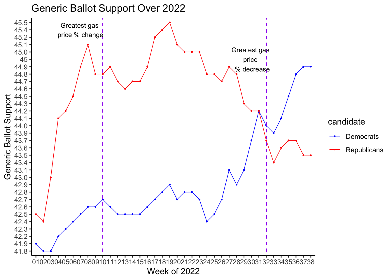
While gas prices as a shock could also be considered an economic factor, I wanted to include them in my model just to determine if they would make a difference at all. From the weekly gas price data, I used the maximum and minimum values of change in gas prices within a given year as my measurement, in order to try to capture what might be the most shocking value, or a value that could impact voter behavior. For this, maximum values are positive changes (increases) in gas prices, and minimum values are negative changes (decreases) in gas prices.
gas <- gas %>%
  mutate(date = mdy(date)) %>%
  mutate(year = substr(date, 1, 4)) %>%
  mutate(week = strftime(date, format = "%V")) %>%
  mutate(month = strftime(date, format = "%m")) %>%
  mutate(avg_change = 100*
           ((avg_gasprice - lag(avg_gasprice)) / (lag(avg_gasprice))))

gas$avg_change[is.na(gas$avg_change)] <- 0
gas$year <- as.character(gas$year)

aggregate(gas$avg_change, by = list(gas$year), max)
## Group.1 x
## 1 1990 4.534005
## 2 1991 1.964453
## 3 1992 2.436647
## 4 1993 4.297994
## 5 1994 2.389381
## 6 1995 1.880036
## 7 1996 3.156146
## 8 1997 2.933780
## 9 1998 3.000000
## 10 1999 6.391347
## 11 2000 5.629838
## 12 2001 4.735547
## 13 2002 6.905594
## 14 2003 7.375538
## 15 2004 5.260304
## 16 2005 17.586207
## 17 2006 5.832629
## 18 2007 5.119597
## 19 2008 5.126096
## 20 2009 7.795958
## 21 2010 3.571429
## 22 2011 6.083412
## 23 2012 3.905359
## 24 2013 5.391719
## 25 2014 2.145663
## 26 2015 6.046312
## 27 2016 6.518197
## 28 2017 11.671530
## 29 2018 1.967335
## 30 2019 3.996865
## 31 2020 4.366347
## 32 2021 5.277889
## 33 2022 13.691796gas2 <- aggregate(avg_change ~ year, data = gas, max)
data.frame(gas2)## year avg_change
## 1 1990 4.534005
## 2 1991 1.964453
## 3 1992 2.436647
## 4 1993 4.297994
## 5 1994 2.389381
## 6 1995 1.880036
## 7 1996 3.156146
## 8 1997 2.933780
## 9 1998 3.000000
## 10 1999 6.391347
## 11 2000 5.629838
## 12 2001 4.735547
## 13 2002 6.905594
## 14 2003 7.375538
## 15 2004 5.260304
## 16 2005 17.586207
## 17 2006 5.832629
## 18 2007 5.119597
## 19 2008 5.126096
## 20 2009 7.795958
## 21 2010 3.571429
## 22 2011 6.083412
## 23 2012 3.905359
## 24 2013 5.391719
## 25 2014 2.145663
## 26 2015 6.046312
## 27 2016 6.518197
## 28 2017 11.671530
## 29 2018 1.967335
## 30 2019 3.996865
## 31 2020 4.366347
## 32 2021 5.277889
## 33 2022 13.691796colnames(gas2)[2] ="maxchange"
gas3 <- gas %>%
group_by(year) %>%
filter(avg_change == min(avg_change)) %>%
select(year, avg_change)
colnames(gas3)[2] ="minchange"
gas3 <- gas3%>%
drop_na()
gas2 <- gas2%>%
drop_na()
gasall <- gas2 %>%
left_join(gas3, by=c("year"))
gasall$year <- as.numeric(gasall$year)combineddata <- read_csv("/Users/claireduncan/Downloads/combineddata.csv")## Rows: 168 Columns: 16## ── Column specification ────────────────────────────────────────────────────────
## Delimiter: ","
## chr (5): st_cd_fips, state, rep_status, dem_status, winner_party
## dbl (11): district, cvap, year, x1, dem_votes_major_percent, rep_votes_major...##
## ℹ Use `spec()` to retrieve the full column specification for this data.
## ℹ Specify the column types or set `show_col_types = FALSE` to quiet this message.dat <- combineddata %>%
left_join(gasall, by = c("year"))However, in the model I have been using, as it’s based solely on the 2014 and 2018 midterms, there were only 2 data points that could be used for both minimum and maximum values. This is not a good model due to the severe data limitations, and it does not give a predictive value that makes sense. For the Democratic vote percent, the minimum value was noted as NA because of singularities. The maximum change variable was statistically significant, as an increase in gas prices was correlated with a -13.177% decrease in vote percent. I tried to figure out why the minimum value would not show up - but it does when I take the maximum value out of the equation. So I ended up running two models, one using the minimum and one using the maximum. The one with the minimum gave a correlation of 0.961, indicating decreases in gas prices were associated with about a percent increase in Democratic vote share. I also ran two models for Republican vote share, given the same problem occurred. I think this is because of the data I am using. For the Republican vote percent, the positive change in gas prices was correlated with a 13.177 increase in vote, inverse of the Democratic vote relationship, which was statistically significant. The correlation between Republican vote share and minimum change was -0.961, indicating that smaller gas price changes had a negative effect on voting for Republicans, which was statistically significant.
D_lm_max <- lm(dem_votes_major_percent ~ maxchange + incumbency + avg_rating + turnout, data = dat)
stargazer(D_lm_max, type='text')
##
## ===============================================
## Dependent variable:
## ---------------------------
## dem_votes_major_percent
## -----------------------------------------------
## maxchange -13.177***
## (3.243)
##
## incumbency -0.020
## (0.438)
##
## avg_rating -2.685***
## (0.107)
##
## turnout 0.023
## (0.027)
##
## Constant 86.519***
## (7.698)
##
## -----------------------------------------------
## Observations 168
## R2 0.802
## Adjusted R2 0.797
## Residual Std. Error 2.414 (df = 163)
## F Statistic 164.974*** (df = 4; 163)
## ===============================================
## Note: *p<0.1; **p<0.05; ***p<0.01prob_D_lm_max <- predict(D_lm_max, newdata =
data.frame(avg_rating = 3.3, turnout = 48.61, incumbency = 1, maxchange = 13.691796), type="response", interval="predict")
prob_D_lm_max## fit lwr upr
## 1 -101.6753 -176.498 -26.85259D_lm_min <- lm(dem_votes_major_percent ~ minchange + incumbency + avg_rating + turnout, data = dat)
stargazer(D_lm_min, type='text')##
## ===============================================
## Dependent variable:
## ---------------------------
## dem_votes_major_percent
## -----------------------------------------------
## minchange 0.961***
## (0.236)
##
## incumbency -0.020
## (0.438)
##
## avg_rating -2.685***
## (0.107)
##
## turnout 0.023
## (0.027)
##
## Constant 63.924***
## (2.323)
##
## -----------------------------------------------
## Observations 168
## R2 0.802
## Adjusted R2 0.797
## Residual Std. Error 2.414 (df = 163)
## F Statistic 164.974*** (df = 4; 163)
## ===============================================
## Note: *p<0.1; **p<0.05; ***p<0.01prob_D_lm_min <- predict(D_lm_min, newdata =
data.frame(avg_rating = 3.3, turnout = 48.61, incumbency = 1, minchange =-3.6736641), type="response", interval="predict",)
prob_D_lm_min## fit lwr upr
## 1 52.62306 47.82112 57.42499R_lm_max <- lm(rep_votes_major_percent ~ maxchange + incumbency + avg_rating + turnout, data = dat)
stargazer(R_lm_max, type='text')##
## ===============================================
## Dependent variable:
## ---------------------------
## rep_votes_major_percent
## -----------------------------------------------
## maxchange 13.177***
## (3.243)
##
## incumbency 0.020
## (0.438)
##
## avg_rating 2.685***
## (0.107)
##
## turnout -0.023
## (0.027)
##
## Constant 13.481*
## (7.698)
##
## -----------------------------------------------
## Observations 168
## R2 0.802
## Adjusted R2 0.797
## Residual Std. Error 2.414 (df = 163)
## F Statistic 164.974*** (df = 4; 163)
## ===============================================
## Note: *p<0.1; **p<0.05; ***p<0.01prob_R_lm_max <- predict(R_lm_max, newdata =
data.frame(avg_rating = 3.3, turnout = 48.61, incumbency = 0, maxchange = 13.691796), type="response", interval="predict",)
prob_R_lm_max## fit lwr upr
## 1 201.6551 126.8917 276.4184R_lm_min <- lm(rep_votes_major_percent ~ minchange + incumbency + avg_rating + turnout, data = dat)
stargazer(R_lm_min, type='text')##
## ===============================================
## Dependent variable:
## ---------------------------
## rep_votes_major_percent
## -----------------------------------------------
## minchange -0.961***
## (0.236)
##
## incumbency 0.020
## (0.438)
##
## avg_rating 2.685***
## (0.107)
##
## turnout -0.023
## (0.027)
##
## Constant 36.076***
## (2.323)
##
## -----------------------------------------------
## Observations 168
## R2 0.802
## Adjusted R2 0.797
## Residual Std. Error 2.414 (df = 163)
## F Statistic 164.974*** (df = 4; 163)
## ===============================================
## Note: *p<0.1; **p<0.05; ***p<0.01prob_R_lm_min <- predict(R_lm_min, newdata =
data.frame(avg_rating = 3.3, turnout = 48.61, incumbency = 0, minchange =-3.6736641), interval="predict", type="response")
prob_R_lm_min## fit lwr upr
## 1 47.35673 42.50972 52.20374Shocks are hard to predict, which my prediction model clearly demonstrated. I used the high increase value of this year in gas prices - which in March was a 13.69% change. The smallest decrease value of this year was -3.67%. The prediction for Democrat vote share using the gas price decrease was 52.62%. The prediction using the gas price increase was -101.67% which obviously does not make sense. The prediction for Republican vote share using the gas price decrease was 47.35%. The prediction for Republican vote share using the gas price increase was 201.65%, which also doesn’t make sense. I believe that the problems with the maximum increase in gas prices are due to this year’s huge shock of gas prices, and the outlier of the 13% change.
I will not be using gas prices in my final model and will have to do more data analysis and cleaning work in order to obtain more values for my prediction model when I make my final analysis. Also for this model, I did not use a pooled model considering the focus of my project and data presentation was on gas prices and even the limitations of data within that.